 abrightersun.de
 I am currently building a little recordable music chip, like the Nuvoton ISD chips, but using nothing more than a microcontroller. Since these chips have quite little flash memory, I need to compress the audio samples. One way to do that is differential pulse-code modulation. It's a very low-complexity linear encoding, which encodes consecutive values as their difference.
The algorithm
The encoding E(S, x) turns an input signal x (the model) into a series y of symbols, taken from the symbol table S, the set {s0, s1, ..., sn − 1} . Each symbol represents a specific difference.
Q(S, q) returns the symbol of set S that matches the difference q best. One way to define a cost model is to compute the absolute error between the difference q and each si.
Decoding the series y of symbols turns it back into the decoded output signal (the prediction) p:
Iff D(E(W))=W, then the coding is lossless. Whether this is the case depends on the input wave and the used code table. To encode all possible input signals the symbol table has to be just as big as the dynamic range of the model, e.g. 8-bit integer audio needs a symbol table of 256 entries to ensure lossless coding.
But we are not restricted to using a full-sized symbol table. We can shrink it to a suitable subset and choose appropriate symbols according to a cost model, such that each difference maps to a best-fitting symbol. Sierra for example used a 4-bit symbol table to encode 8-bit music and voice data to achieve a compression of 2:1.
Implementation
Straight-forward implementation of a DPCM codec in Python:
import numpy as np

class DPCM(object):

    def __init__(self, diff_table):
        self.diff_table = array(diff_table)

    def encode(self, wave):
        if len(wave.shape)==2:
            return np.vstack([self.encode(wave[:,0]),self.encode(wave[:,1])]).T
        symbols = np.zeros(len(wave), dtype=np.uint)
        prediction = 0
        for i, model in enumerate(wave):
            predictions = prediction + self.diff_table
            abs_error = np.abs(predictions - model)
            diff_index = np.argmin(abs_error)
            symbols[i] = diff_index
            prediction += self.diff_table[diff_index]
        return symbols

    def decode(self, symbols):
        if len(symbols.shape)==2:
            return np.vstack([self.decode(symbols[:,0]),self.decode(symbols[:,1])]).T
        wave = np.zeros(len(symbols), dtype=np.double)
        prediction = 0
        for i, diff_index in enumerate(symbols):
            prediction += self.diff_table[diff_index]
            wave[i] = prediction
        return wave

# Example usage:
wave = 128*np.cos(2*np.pi*np.arange(100)/100.)
wave = np.vstack([wave,wave]).T
half_table = np.array([1,2,4,8,16,32,64,128])
diff_table = np.hstack([half_table,-half_table])
codec = DPCM(diff_table)
dpcm_wave = codec.decode(codec.encode(wave))
Encoding signals longer than a few thousand samples takes a long time using this code. I implemented it also in Cython and got a 355x speed increase over pure Python. You may download an archive containing the full code at the end of the article.
Modulation transfer function
One interesting property is how a (co-) sine wave of varying frequency gets processed by the encoder. To analyze this, waves spanning the whole frequency range from DC up to the Nyquist frequency are generated, encoded, again decoded and their spectral power measured. A perfect (lossless) system should transfer each frequency without alteration either in phase or in magnitude. The modulation transfer function evaluates only the magnitude portion by setting the output power of a system into relation of the input power.
Using a naive 4-bit symbol table
and generating 8-bit signed integer signals results in the following transfer function:
Modulation transfer function of DPCM encoded sine waves of varying frequencies. For each generated signal the output spectral power is measured and related to its input power. Ideally, each frequency should be transferred without change in magnitude.
The process is obviously not lossless for S0, some frequencies are even attenuated by more than 20 dB. Interestingly, the high frequencies near the Nyquist frequency get transferred rather well.
We can do better by adapting the symbol table. Instead of choosing consecutive numbers, let's use a base-2 exponential series:
This accomodates for both small and large swings in the ouput. High frequencies should benefit from that, since their large deltas could not be encoded directly by S0. The modulation transfer function looks much better now:
Modulation transfer function of sine waves of varying frequencies, encoded using a base-2 exponential symbol table.
The worst attenuation is now around -1 dB instead of -20 dB. But this is only half the picture. Another property is the frequency response of the encoding. Using a lossy symbol table introduces artifacts that were not present in the original data. Consider the frequency response of a PCM sine sweep:
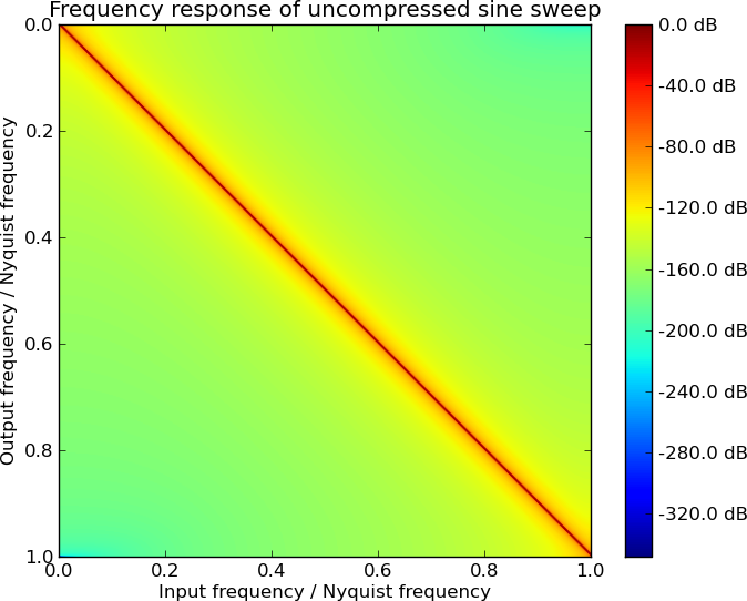
The response is defined by one large peak along the diagonal, meaning the excitation frequency results in the same output frequency peak and nothing more.
Now the sine sweep encoded with Sb2:

While the modulation transfer function looks well enough, there is a lot of leakage into other frequencies (and some repeating harmonics). But a lot of the spectral power lies below the noise floor of -50 dB (see SNR of digital signals). Zooming into the relevant value range reveals the following picture:

It doesn't look so horrible now. Most of the introduced noise lies below -20 dB. One exemplary vertical slice of the figure above shows how the spectral power is distributed in detail:

The spectrum is made up of repeating small peaks uniformly distributed across the whole spectral range. This means a lot of harmonics which result in a "raspy" sound.
Adapting the symbol table
Up until now the choice of the coding symbols was independent from the actual encoded sound. Looking at the peaks of a histogram of the differences between samples of a chosen audio file reveals the most often appearing differences. This enables tailoring the symbol set to the data. To assess the quality an objective error metric is needed. Both the RMS (root mean square) and the average SNR are useful tools:
While the RMS error the describes the absolute error between the raw and encoded signal, SNR gives an idea how much "space" there is between the signal and the noise floor.
The following two sound bites will be used: JFK's famous words "Ich bin ein Berliner" and John Williams' "Raider's March" of Indiana Jones fame. Both files have differing spectra and dynamic ranges serving as examples for typical music and voice data.
First the plot of the difference histograms:

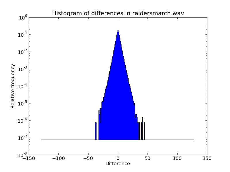
The spread of both samples is relatively tight, ≈ ±25 for JFK, ≈ ±50 for raider's march. Interestingly, the difference frequency falls exponentially with the difference magnitude.
Considering these (similar) distributions, I built the empirical adapted symbol table Sa:
Encoding both samples with the diverse constructed symbol tables yielded the following results:
| File | Symbol table | \(\text{RMS}(D(E(x))-x)\) | \(\overline{\text{SNR}}\) |
|---|---|---|---|
| JFK | \(S_0\) | 2.091 | 22.12 dB |
| JFK | \(S_{b2}\) | 0.768 | 25.50 dB |
| JFK | \(S_a\) | 0.413 | 29.07 dB |
| Raider's March | \(S_0\) | 1.290 | 21.59 dB |
| Raider's March | \(S_{b2}\) | 0.870 | 22.86 dB |
| Raider's March | \(S_a\) | 0.651 | 23.82 dB |
The adapted symbol set works best, as the RMS error and SNR show. But while JFK's error is quartered, it is only halved for raider's march. This is consistent with the more diverse differences occuring in the music piece, due to the higher dynamic range of the signal.
Listening to the results
Original:
JFK
Raider's march
Encoded using S0:
JFK
Raider's march
Encoded using Sb2:
JFK
Raider's march
Encoded using Sa:
JFK
Raider's march
Without using headphones, they all sound the same to me. Which means DPCM coding is a great contestant for my microcontroller-based sound chip. Nevertheless, I will still research other interesting approaches, like µ-law encoding, linear predictive coding, vocoders and ADPCM (obviously).
Download
Simple implementation of an DPCM codec, both in pure Python and in Cython: dpcm.zip.